使用R语言tidyverse包轻松实现PCA分析

在本文中,我们将使用主成分分析(PCA)技术对乳腺癌数据集进行分析,并通过数据可视化来展示分析结果。

数据预处理

首先,我们清除环境中的所有变量,然后加载必要的库并读取数据。

rm(list=ls())library(tidyverse)library(broom)library(cowplot)biopsy <- read.csv('biopsy.csv', row.names = 1)

主成分分析(PCA)

接下来,我们对数值型数据进行标准化处理,并进行PCA。

pca_fit <- biopsy %>%   select(where(is.numeric)) %>% # retain only numeric columns  prcomp(scale = TRUE) # do PCA on scaled datapca_fit
# Standard deviations (1, .., p=9):#   [1] 2.4288885 0.8808785 0.7343380 0.6779583 0.6166651 0.5494328 0.5425889 0.5106230 0.2972932# # Rotation (n x k) = (9 x 9):#   PC1         PC2          PC3         PC4         PC5         PC6          PC7         PC8          PC9# clump_thickness      -0.3020626 -0.14080053  0.866372452  0.10782844 -0.08032124 -0.24251752 -0.008515668 -0.24770729  0.002747438# uniform_cell_size    -0.3807930 -0.04664031 -0.019937801 -0.20425540  0.14565287 -0.13903168 -0.205434260  0.43629981  0.733210938# uniform_cell_shape   -0.3775825 -0.08242247  0.033510871 -0.17586560  0.10839155 -0.07452713 -0.127209198  0.58272674 -0.667480798# marg_adhesion        -0.3327236 -0.05209438 -0.412647341  0.49317257  0.01956898 -0.65462877  0.123830400 -0.16343403 -0.046019211# epithelial_cell_size -0.3362340  0.16440439 -0.087742529 -0.42738358  0.63669325  0.06930891  0.211018210 -0.45866910 -0.066890623# bare_nuclei          -0.3350675 -0.26126062  0.000691478  0.49861767  0.12477294  0.60922054  0.402790095  0.12665288  0.076510293# bland_chromatin      -0.3457474 -0.22807676 -0.213071845  0.01304734 -0.22766572  0.29889733 -0.700417365 -0.38371888 -0.062241047# normal_nucleoli      -0.3355914  0.03396582 -0.134248356 -0.41711347 -0.69021015  0.02151820  0.459782742 -0.07401187  0.022078692# mitoses              -0.2302064  0.90555729  0.080492170  0.25898781 -0.10504168  0.14834515 -0.132116994  0.05353693 -0.007496101

可视化主成分分析结果

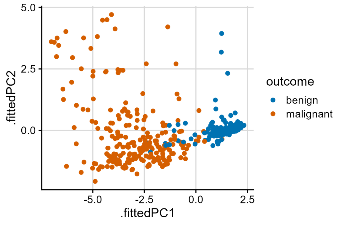
我们使用 ggplot2 包将 PCA 的结果可视化。首先是主成分得分图,显示了前两个主成分的得分,并根据样本的结果进行着色。

pca_fit %>%augment(biopsy) %>%ggplot(aes(.fittedPC1, .fittedPC2, color = outcome)) +geom_point(size = 1.5) +scale_color_manual(  values = c(malignant = "#D55E00", benign = "#0072B2")) +theme_half_open(12) +background_grid()

主成分载荷图

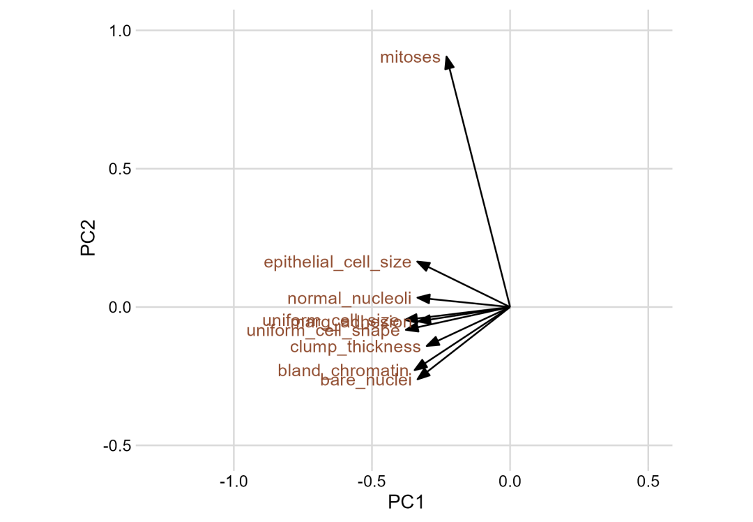
接下来,我们提取并绘制旋转矩阵,用箭头表示每个变量在前两个主成分上的载荷。

# 定义箭头样式arrow_style <- arrow(angle = 20, ends = "first", type = "closed", length = grid::unit(8, "pt"))
# 绘制旋转矩阵pca_fit %>%tidy(matrix = "rotation") %>%pivot_wider(names_from = "PC", names_prefix = "PC", values_from = "value") %>%ggplot(aes(PC1, PC2)) +geom_segment(xend = 0, yend = 0, arrow = arrow_style) +geom_text(  aes(label = column),  hjust = 1, nudge_x = -0.02,  color = "#904C2F") +xlim(-1.25, .5) + ylim(-.5, 1) +coord_fixed() +theme_minimal_grid(12)

主成分解释方差

最后,我们绘制各主成分解释方差的柱状图,以展示每个主成分对总方差的贡献。

pca_fit %>%tidy(matrix = "eigenvalues") %>%ggplot(aes(PC, percent)) +geom_col(fill = "#56B4E9", alpha = 0.8) +scale_x_continuous(breaks = 1:9) +scale_y_continuous(  labels = scales::percent_format(),  expand = expansion(mult = c(0, 0.01))) +theme_minimal_hgrid(12)

原创文章,作者:速盾高防cdn,如若转载,请注明出处:https://www.sudun.com/ask/79114.html

(0)
速盾高防cdn的头像速盾高防cdn
上一篇 2024年5月30日 下午5:44
下一篇 2024年5月30日 下午5:51

相关推荐

发表回复

您的电子邮箱地址不会被公开。 必填项已用 * 标注