
这次利用NCEP/NCAR的再分析数据(https://psl.noaa.gov/data/gridded/data.ncep.reanalysis.html)绘制风场。数据是来自1991年至2020年的长期月平均值(Long term monthly means, derived from years 1991 to 2020),纬向风数据和经向风数据为两个单独的文件,其中纬向风数据下载地址为:
https://downloads.psl.noaa.gov/Datasets/ncep.reanalysis/Monthlies/surface_gauss/uwnd.10m.mon.ltm.1991-2020.nc经向风数据下载地址为:
https://downloads.psl.noaa.gov/Datasets/ncep.reanalysis/Monthlies/surface_gauss/vwnd.10m.mon.ltm.1991-2020.nc首先导入数据处理与绘图的库
import numpy as npimport matplotlib.pyplot as pltimport xarray as xrimport cartopy.crs as ccrsimport geopandas as gpd
读取并查看数据
diri = "C:/Rmet/data/"filiu = "uwnd.10m.mon.ltm.1991-2020.nc" # wind of U componentfiliv = "vwnd.10m.mon.ltm.1991-2020.nc" # wind of V componentfu = xr.open_dataset(diri + filiu)fv = xr.open_dataset(diri + filiv)
数据读取后,会给出一个警告信息,如下:
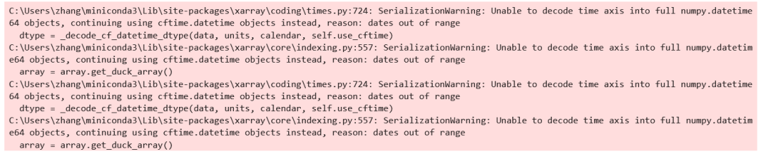
以上的一些警告信息,如 SerializationWarning: Unable to decode time axis into full numpy.datetime64 objects, continuing using cftime.datetime objects instead, reason: dates out of range。
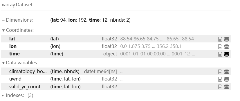
接下来,查看数据,输入:
fu返回如下结果
选定研究区范围的数据
xmin, xmax, ymin, ymax = 70, 180, 0, 60x = fu.coords["lon"]y = fu.coords["lat"]fu = fu.loc[dict(lon = x[(x >= xmin) & (x <= xmax)],lat = y[(y >= ymin) & (y <= ymax)])]fv = fv.loc[dict(lon = x[(x >= xmin) & (x <= xmax)],lat = y[(y >= ymin) & (y <= ymax)])]# 生成数据的坐标矩阵Lon, Lat = np.meshgrid(fu.coords["lon"], fu.coords["lat"])
查看时间维度
f.coords['time']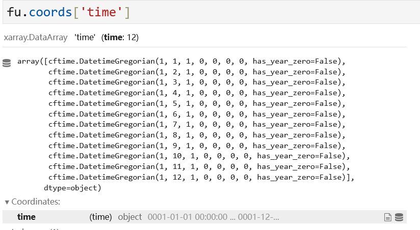
数据在时间上一共有12个月。在python里面,数据的索引是从0开始的,因此,假如我们要选出4月的数据,代码如下:
indTime = 3 # time index. AprilU = fu['uwnd'].isel(time = indTime)V = fv['vwnd'].isel(time = indTime)
从高德读取中国地图矢量文件
#diriMap = "C:/Rmet/data/ChinaMap/CHN_amap.shp"diriMap = "https://geo.datav.aliyun.com/areas_v3/bound/100000.json"cmap = gpd.read_file(diriMap)cmap
绘图
# plotdata_crs = ccrs.PlateCarree() # 设定坐标系fig = plt.figure(figsize=(8, 5)) # 设置图片大小# The projection argument is used when creating plots and determines the projection of the resulting plotax = fig.add_subplot(1, 1, 1, projection = data_crs)ax.set_extent([70, 180, 0, 60], crs = data_crs) # 限定绘图范围ax.coastlines(linewidth = 0.6)#ax.stock_img() # Add a standard image to the mapax.add_geometries(cmap['geometry'], crs = data_crs, fc = "none",edgecolor = "red", linewidth = 0.6)# add gridlinesax.gridlines(crs = data_crs,draw_labels = {"bottom": "x", "left": "y", "right": "y"},rotate_labels = False,xlocs = np.arange(70, 181, 10),ylocs = np.arange(0, 61, 10),x_inline = False, y_inline = False,linewidth=0.5, linestyle='--', color='black')ax.set_title("April mean wind of 10m from the NCEP Reanalysis",loc = "left")# add wind vectornxy = 2 # skip 2 gridsquiver = ax.quiver(Lon[::nxy, ::nxy], Lat[::nxy, ::nxy],U[::nxy, ::nxy], V[::nxy, ::nxy],transform = data_crs)# 设置风速图例ax.quiverkey(quiver, 0.93, 1.03, 5, "5m/s",labelpos='E', coordinates='axes')plt.savefig('C:/Rmet/figures/Wind.png', dpi = 600)plt.show()
绘图效果如下

原创文章,作者:guozi,如若转载,请注明出处:https://www.sudun.com/ask/88208.html